Model Editor

This month we are going to discuss the Cincom® ObjectStudio® Model Editor.  The Model Editor should not be confused with the Modeling Tool.  The Model Editor helps you to develop a calculation model that you can use in your application afterwards.

You can always develop such a model in plain Smalltalk, but the Model Editor helps you to prototype the model and gives you a graphical preview of it. In the late 1980’s, a Dutch company used the Model Editor extensively to create a tactical battlefield command and control system to render all kinds of tactical maps.

As an example, we’ve created a very simple model to calculate the break-even point. We’ve added some variables to the model and given them some values and formulas for our prototype:

• fixedCost -> 4521 (the cost even if we don’t produce a unit).
• variableCost -> 384 (the additional cost for each unit produced).
• quantity -> the number of units produced and sold.
• unitPrice -> 500 (the sale price of one unit).
• totalVariableCost -> quantity * variableCost
• totalCost -> fixedCost + totalVariableCost
• totalRevenue -> quantity * unitPrice
• profitLoss -> totalRevenue – totalCost
• marker -> (profitLoss > 0) ifTrue: [totalRevenue] ifFalse: [0] (This will create a vertical line at the break-even point).

When you open a new model, you can start entering variables. A window pops up where you define a variable.

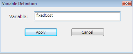
When you apply, the variable is stored and you can enter a new one. This is repeated until you press cancel on the Variable Definition window. The same process can be started in a later phase by choosing the New… submenu in the Variable menu.

To assign a value or formula to a variable, you simply select the variable in the inputs, intermediates or outputs list and type the assignment in the Formula text field.  As long as a variable has no value or formula assigned it remains in the inputs list. After a variable gets a value or formula, the variable moves to the outputs list. If the variable is used in another formula for another variable, it’s again moved, but this time to the intermediates list.

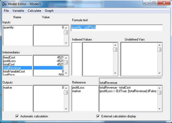
Once you’ve entered the base for your model, you go to the Graph-Setup option:

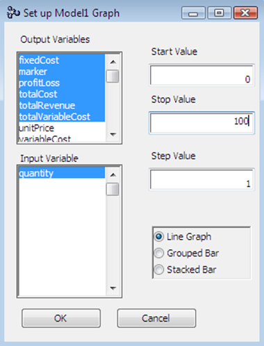
You select which values you want to see on the graph, and you select an input variable. Enter Start-Stop-Step values for the input variable and a graph type. When you press OK, you’ll get a very basic graph of your model:

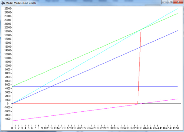
• The pink line is the profit/loss value.
• The red line is the marker.
• The blue horizontal line is the fixed cost.
• The dark-blue line is the variable cost.
• The light-blue line is the total revenue.
• The green line is the total cost.

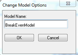
Before we save the model, we’ll first give it a useful name with the File – Change Options menu.  Let’s call our example BreakEvenModel.

How do we use this newly created model in your application?

You can create a wrapper around the model. We create a class named BreakEvenWrapper with ‘model’ as an instance variable. To create an instance of the wrapper, we have:

In ObjectStudio, System is a global dictionary that contains global variables and classes from the ObjectStudio namespace. So with System at: #BreakEvenModel, we get our unique instance of the BreakEvenModel.

Now we create some getters and accessors to the model.

Now you can write code like:

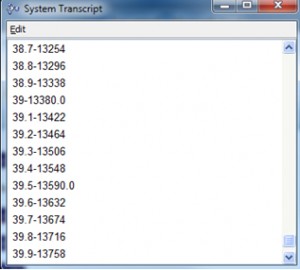
In a transcript, this looks like: